Publishing Results
Click here to find out how to optimise dSNAP and PolySNAP graphics displays for publication.
Compare programs
Click here for an overview comparing dSNAP, PolySNAP and PolySNAP M.


SNAP software is developed by the
Theoretical Crystallography group at the University of Glasgow, and is
exclusively distributed by Bruker AXS.
dSNAP Worked Example
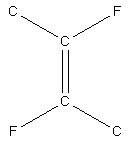
A CSD search for a simple di-fluoroalkene fragment (Fig. 1) returns 58 fragments from 33 structures.
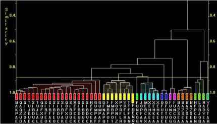
Exporting the geometric information from each fragment and analysing them using dSNAP, an initial dendrogram (Fig. 2a) and 3D plot (Fig. 2b) are obtained.
For Fig. 2a, the lower on the similarity scale two fragments (coloured boxes) are joined by a horizontal tie-bar, the more similar the fragments are.
For Fig. 2b, each sphere represents a fragment, and the further apart two points are, the more different the corresponding fragments are. As a result, similar samples can be seen to ‘clump’ together into clusters. Very similar fragments produce tight clusters, whereas less identical ones give more diffuse groupings. The user is therefore able to tell at a glance quite a lot about the fragments being grouped together by the program, and any outliers are easily spotted. The colours are taken from the dendrogram display, allowing comparison of the results from the two separate analysis methods.
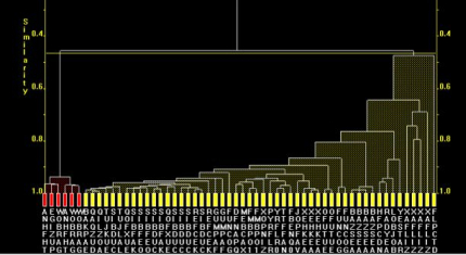
The initial partitioning represents the coarse differences of CIS (yellow) and TRANS (red) versions of the fragment. By further subdividing just the yellow cis group (Fig. 3a and 3b), more detailed differences can be observed.
By studying example fragments from each of these clusters in Mercury, and looking at their orientations overlaid in the 3D Fragment Viewer (Fig. 4), each of these smaller groups can all be justified as being different in terms of their chemical structure, as shown in the table below.
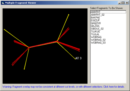
Fig. 1. The di-fluoroalkene fragment used in the search
Exporting the geometric information from each fragment and analysing them using dSNAP, an initial dendrogram (Fig. 2a) and 3D plot (Fig. 2b) are obtained.
Fig. 2a. The dendrogram
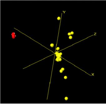
Fig. 2b. The 3-dimensional MMDS plot
Fig. 2b. The 3-dimensional MMDS plot
For Fig. 2a, the lower on the similarity scale two fragments (coloured boxes) are joined by a horizontal tie-bar, the more similar the fragments are.
For Fig. 2b, each sphere represents a fragment, and the further apart two points are, the more different the corresponding fragments are. As a result, similar samples can be seen to ‘clump’ together into clusters. Very similar fragments produce tight clusters, whereas less identical ones give more diffuse groupings. The user is therefore able to tell at a glance quite a lot about the fragments being grouped together by the program, and any outliers are easily spotted. The colours are taken from the dendrogram display, allowing comparison of the results from the two separate analysis methods.
The initial partitioning represents the coarse differences of CIS (yellow) and TRANS (red) versions of the fragment. By further subdividing just the yellow cis group (Fig. 3a and 3b), more detailed differences can be observed.
Fig. 3a. The modified dendrogram of Cis fragments only
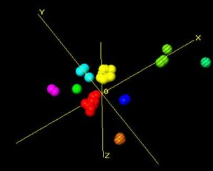
Fig. 3b. The revised 3-dimensional plot
Fig. 3b. The revised 3-dimensional plot
By studying example fragments from each of these clusters in Mercury, and looking at their orientations overlaid in the 3D Fragment Viewer (Fig. 4), each of these smaller groups can all be justified as being different in terms of their chemical structure, as shown in the table below.
Fig. 4. Selected cis- and trans-fragments overlaid
| Colour in Fig. 3a/3b | Form | Description | Number of fragments |
| Red | Trans | Sterically non-constrained; ideal geometry | 3 |
| Yellow | Trans | Sterically onstrained | 3 |
| Green | Cis | All fragments of tetrafluoro-7,7,8,8-tetracyanoquinodimethane | 21 |
| Pale blue | Cis | At least one 3-coordinate carbon R-groups generally to an O atom | 8 |
| Dark blue | Cis | Sterically constrained 7-membered ring | 1 |
| Pink | Cis | Both R-groups are 4-coordinate | 5 |
| Orange (striped) | Cis | Resonant C=C bonds with partial double character | 2 |
| Yellow green (striped) | Cis | Sterically constrained B2 | 2 |
| Green (striped) | Cis | Mislabelled bonds in the database | 4 |
| Blue (striped) | Cis | Bridged 6-membered ring | 3 |
| Purple (striped) | Cis | Bridged 6-membered ring | 1 |
| Next four groups | Cis | Carbon-cluster | 4 |
| Last entry | Cis | Part of a cyclobutene ring | 1 |
In this way a detailed level of analysis can be performed in dSNAP in a minimal amount of time.
Further, more detailed examples can be found in the references linked to on this page.
Further, more detailed examples can be found in the references linked to on this page.